Class 3: Clustering Algorithms for Cybersecurity

Class 3: Clustering Algorithms for Cybersecurity#

Caution

Disclaimer This is an experimental format. The content of this page was adapted from Professor Roman’s Lecture in Fall 2025. Claude 4.5 was used to clean up the audio transcripts and adapt them for this format. AI may make mistakes. If you into any issues please open an Issue or send an email to the TA Sasank

Learning Objectives#

By the end of this session, you will be able to:

Understand the mathematical foundations of clustering algorithms
Apply K-means, GMM, and DBSCAN to cybersecurity data
Recognize when different clustering approaches fail or succeed
Select appropriate clustering methods based on data characteristics
Implement cluster validation techniques

Hint

Follow Along

If you want to execute this on your own you can open the 03-Class 3 [Jupyter Notebook].ipynb in or download it from Canvas and run these on your local machine.
The original video for this lecture is posted here

Note: these links are only accessible for Duke students

Overview#

Alright everyone, welcome to Class 3.

Let’s recap what we’ve covered so far. We’ve learned several supervised methods:

K-Nearest Neighbors - Classification via neighborhood consensus. You look at what’s similar and determine the threat category based on known labeled examples.
Support Vector Machines - Finding optimal decision boundaries in high-dimensional feature spaces for malware classification.
Random Forest - Ensemble learning providing robust classification through multiple decision trees.

What’s the common thread tying all of these together?

Hint

The label issue Supervised methods require extensive labeled training data to distinguish benign from malicious activities.

And that’s the big problem.

Labeling, it turns out, is extremely challenging for cybersecurity. I’m using a 2017 dataset for this class - there are newer ones from 2022 and 2023, but many of these are synthetic datasets created in laboratory settings specifically so people can train models on them

The Reality of Real-World Data#

When you get into production environments, getting labeled data is incredibly difficult:

Cyber threats evolve faster than our ability to label them - By the time you’ve identified and labeled a threat, attackers have moved on to new techniques.
Zero-day attacks - These exploit previously unknown vulnerabilities. There are no historical signatures, no labels, nothing to train on.
Class imbalance - Attacks represent rare events in typical network traffic. You might have millions of benign events and only a handful of attacks.
Manual labeling is expensive - It’s time-intensive and requires expert domain knowledge. You need security analysts spending hours examining logs to determine what’s actually malicious.

The “Unknown Unknowns” Framework#

Let me frame this using a concept from intelligence analysis:

Known Knowns - These are documented attack signatures, indicators of compromise (IOCs), and established threat patterns with clear detection rules. Your signature-based systems handle these well.
Known Unknowns - These are suspected attack vectors and emerging threats without specific signatures or clear indicators. You know something might be out there, but you don’t know exactly what it looks like.
Unknown Unknowns - These are completely novel attack methods, threat actors, and exploitation techniques never before observed. This is where traditional security fails completely.

Why Traditional Detection is Failing#

Let me walk you through the cybersecurity imperative here:

Signature-Based Detection is fundamentally reactive. It requires known attack patterns and signatures. It completely fails against novel threats and sophisticated evasion techniques.
Advanced Persistent Threats (APTs) run long-term, stealthy campaigns using legitimate administrative tools and techniques specifically to avoid detection.
“Living off the Land” (LotL) Attacks abuse legitimate system tools - PowerShell, WMI, PsExec - making detection extremely challenging. These tools are supposed to be there, used by administrators every day.

The critical result?

Important

The Limitation of Traditional Systems Traditional antivirus and intrusion detection systems consistently miss sophisticated threats that blend with normal administrative activities.

Real-World Impact#

Let me give you some real examples:

NotPetya (2017)#

Used legitimate PsExec for lateral movement while masquerading as ransomware. It evaded signature-based detection during initial propagation phases because it was using a tool that was supposed to be there.

SolarWinds (2020)#

Supply chain attack that hid malicious code within normal software update processes. It remained undetected for months because it came through legitimate channels. How do you detect a threat when it’s delivered by your trusted update system?

Volt Typhoon (2023)#

This PRC-sponsored group used Living off the Land techniques for over five years, completely bypassing traditional detection systems. Five years! Using legitimate tools the entire time.

The critical pattern across all these attacks is they successfully bypassed signature-based detection by leveraging legitimate tools and processes. This demonstrates the urgent need for behavioral analysis approaches.

We need to stop asking

Is this a known attack?

and start asking

What does normal look like?

Enter Unsupervised Learning#

This is where unsupervised learning comes in. Unsupervised learning is great for:

Pattern Discovery - Algorithms find hidden patterns and structures in data without requiring pre-labeled examples.
Normality Modeling - We shift focus from attack classification to establishing baselines of normal behavior.
Deviation Detection - We identify significant departures from established behavioral baselines.

The key insight: instead of asking “Is this a known attack?”, we ask “Does this behavior deviate significantly from established norms?”

Hint

Ask Different Questions “Does this behavior deviate significantly from established norms?”

Clustering Approach#

The core function of unsupervised learning is to identify “normal” by grouping (or clustering) similar data points, allowing anomalies to stand out.

Think about normal behaviors in your network:

Consistent web browsing patterns
Regular email communication flows
Standard file transfer behaviors
Routine system administration tasks

When you establish these patterns, attacks stand out. Abnormal behavior is not in the same cluster in your parameter space as your normal behavior. Examples include:

Unusual communication patterns, like connections to command and control servers
Abnormal resource usage, like unexpected crypto-mining activity
Strange temporal patterns, like logins at odd hours when users are typically offline
Outlier behaviors that don’t align with any established norms

These abnormal behaviors may even be context dependent. Normal for someone in finance but not sompeone in operations.

Clustering Philosophies#

Today we’re going to cover three fundamentally different approaches to clustering:

Centroid-Based: K-means#

Philosophy: Groups form around central points.
Assumption: Clusters are spherical and similarly sized.
Best for: Discovering well-separated, distinct attack types or user behavior profiles.

Think of it like this: K-means says “every cluster has a center, and things near that center belong together.” It’s fast, it’s simple, it’s intuitive.

Distribution-Based: Gaussian Mixture Models (GMM)#

Philosophy: Data originates from a mixture of probability distributions.
Assumption: Clusters can be elliptical and probabilistic, allowing for overlap.
Best for: Modeling uncertain classifications or overlapping behavioral patterns.

The key difference is that GMM doesn’t just say “you’re in cluster A or cluster B” - it says “you’re 70% likely to be in cluster A and 30% likely to be in cluster B.” It gives you probability, uncertainty quantification.

Density-Based: DBSCAN#

Philosophy: Groups are defined by regions of high data point density.
Assumption: Clusters can be arbitrary shapes, with automatic noise detection.
Best for: Identifying irregular attack patterns and automatically discerning anomalies from noise without knowing the number of clusters ahead of time.

Why this matters: DBSCAN doesn’t care about cluster shape. It finds dense regions and says “that’s a cluster.” Everything else is just Noise. Potential anomalies.

Each approach offers unique strengths for modeling normal behavior and detecting anomalies in complex cybersecurity datasets.

When you’re doing clustering for cybersecurity, you’re trying to answer three fundamental questions:

Important

The Three Key Questions

How Many Groups?
What Shape?
Which Don’t Belong?

The frist thing you need to do is determine the optimal number of natural behavioral clusters inherent in your network or system data.

Once you do that, the next step is to understand the geometric structure and distribution of these behavioral patterns to accurately model normal activity.

After you have modeled normal activity you need a way to identify data points that do not fit into any established behavioral group, indicating potential anomalies or threats.

Different clustering algorithms answer these questions differently, and that’s what we’re going to explore in the notebook.

Setup and Imports#

Alright, let’s get into the technical details. Now would be a good time to open the notebook (or the lab assignment) and follow along. The below cell involves all of the standard notebook setup that you will need to run this on your own. It is hidden to minimize impact to flow. All code cells can be inspected by clicking on the drop down on the right

Visualizing the Problem#

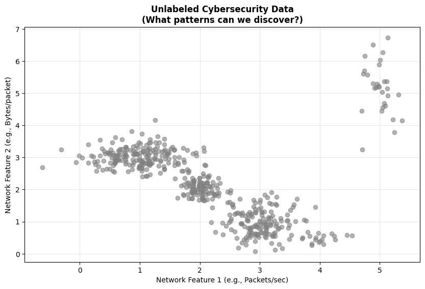
In the notebook, we’re going to start with synthetic data that represents cybersecurity scenarios. This lets us understand the algorithms before applying them to real-world data.

Here’s the challenge we’re facing: most cybersecurity data is unlabeled.

Network traffic logs - You’ve got millions of flows. Which ones are attacks?
User behavior - What constitutes “normal” versus “suspicious”?
System events - Which patterns actually indicate a compromise?

The solution is unsupervised learning to find natural groupings and outliers.

Understanding the Synthetic Data

In the first code cell, we’re creating synthetic cybersecurity-like data to demonstrate the problem:

Normal web traffic - Consistent patterns centered around certain values
Normal email traffic - Different patterns from web traffic
Normal file transfers - Yet another distinct behavioral pattern
DDoS attack - An attack pattern we don’t initially know about
Data exfiltration - Another hidden attack pattern

When we plot this data, you’ll see just gray points. No labels. No indication of what’s what. This is what you’d face in the real world - just data, and you need to figure out what’s normal and what’s not.

../../_images/c7546e4a4031ae7179775994908808dfcb07df072ecb8ad6340038507c85c05a.png

K-means Clustering#

The Mathematical Foundation#

Now let’s talk about K-means. The mathematical objective is to minimize the within-cluster sum of squares (WCSS). This is given by the formula:

\[J = \sum_{i=1}^{k} \sum_{x \in C_i} ||x - \mu_i||^2\]

Where:

\(k\) = number of clusters
\(C_i\) = cluster \(i\)
\(\mu_i\) = centroid of cluster \(i\)
\(||x - \mu_i||^2\) = squared Euclidean distance

The formula might look intimidating, but the concept is simple: for each cluster, you’re summing up the squared distance from every point to that cluster’s center. You want to minimize that total across all clusters.

The algorithm is beautifully simple:

Algorithm Steps:

Initialize: Randomly pick \(k\) points as your initial centroids
Asign: Assign each point to nearest centroid
Update: Update centroids to cluster means: \(\mu_i = \frac{1}{|C_i|} \sum_{x \in C_i} x\)
Repeat: Repeat steps 2-3 until he centroids stop moving, (i.e. convergence)

Watch what happens iteration by iteration. You’ll see the centroids (marked with X’s) start at random positions, then gradually move toward the center of their clusters. The cluster assignments change as the centroids move. Usually, you’ll converge in just a few iterations.

This is the power of K-means - it’s fast and intuitive. You can literally watch it find patterns.

**K-means Algorithm Visualization**
Watch how centroids move and clusters form...
Converged after 6 iterations

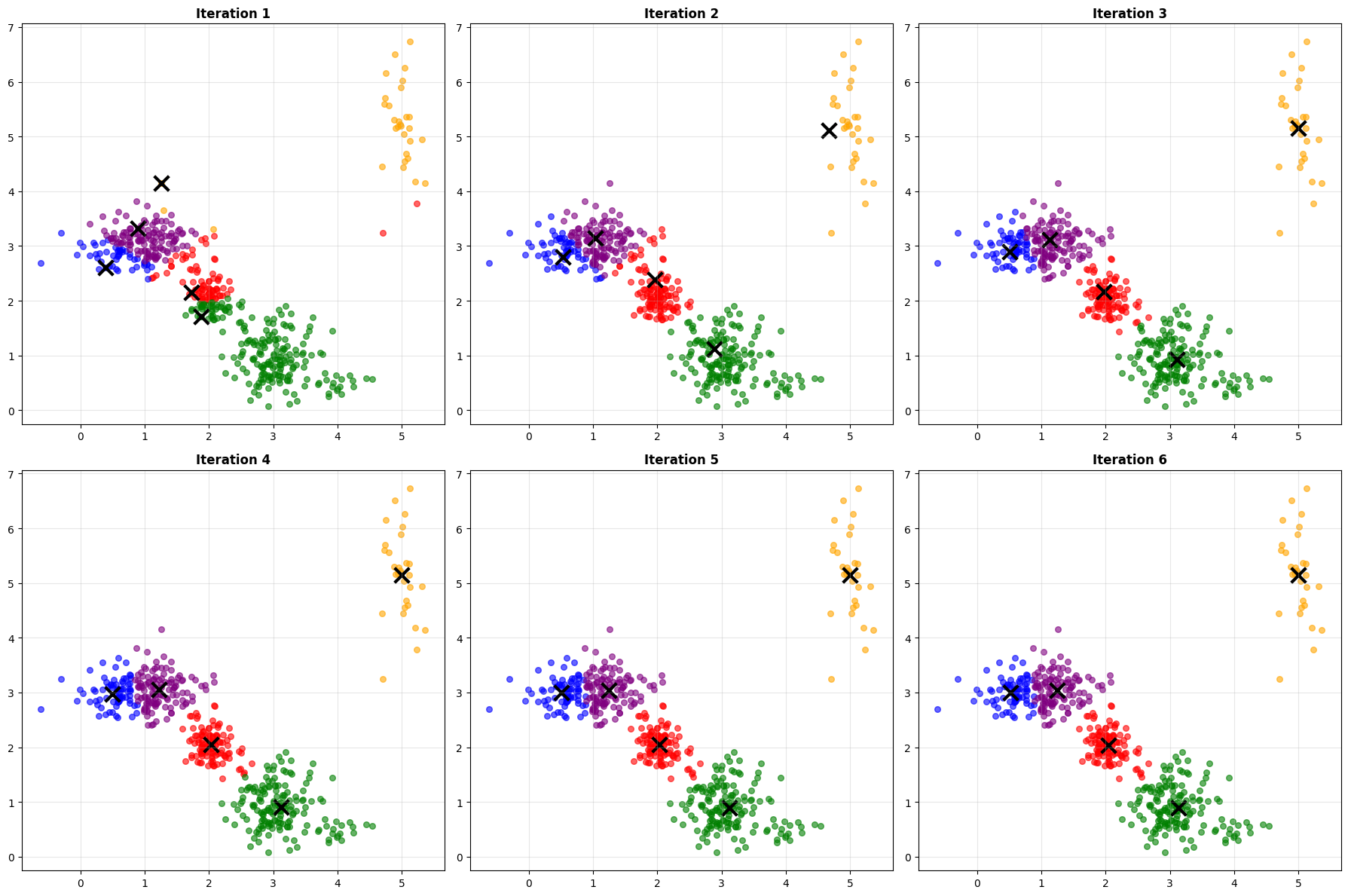
../../_images/6dbf65b2ae75811f8007388c1a81b0f207df53462f3675a5d2eb7435eb270724.png

Final WCSS: 117.54

Key K-Means Hyperparameters#

Like other models, hyperparameter selection influences performance. Below are some of the key hyperparameters involved in K-means.

Parameter	Description	Default	Impact
`n_clusters`	Number of clusters (k)	Must specify	Critical: Determines cluster count
`init`	Centroid initialization	`'k-means++'`	Affects convergence speed/quality
`n_init`	Number of random initializations	`10`	Helps avoid local minima
`max_iter`	Maximum iterations	`300`	Controls convergence
`tol`	Convergence tolerance	`1e-4`	Stopping criteria precision

The Parameter Selection Challenge#

But here’s the big question:

How do we choose \(k\) (number of clusters)?

This is one of the fundamental challenges in unsupervised learning. We have two main methods:

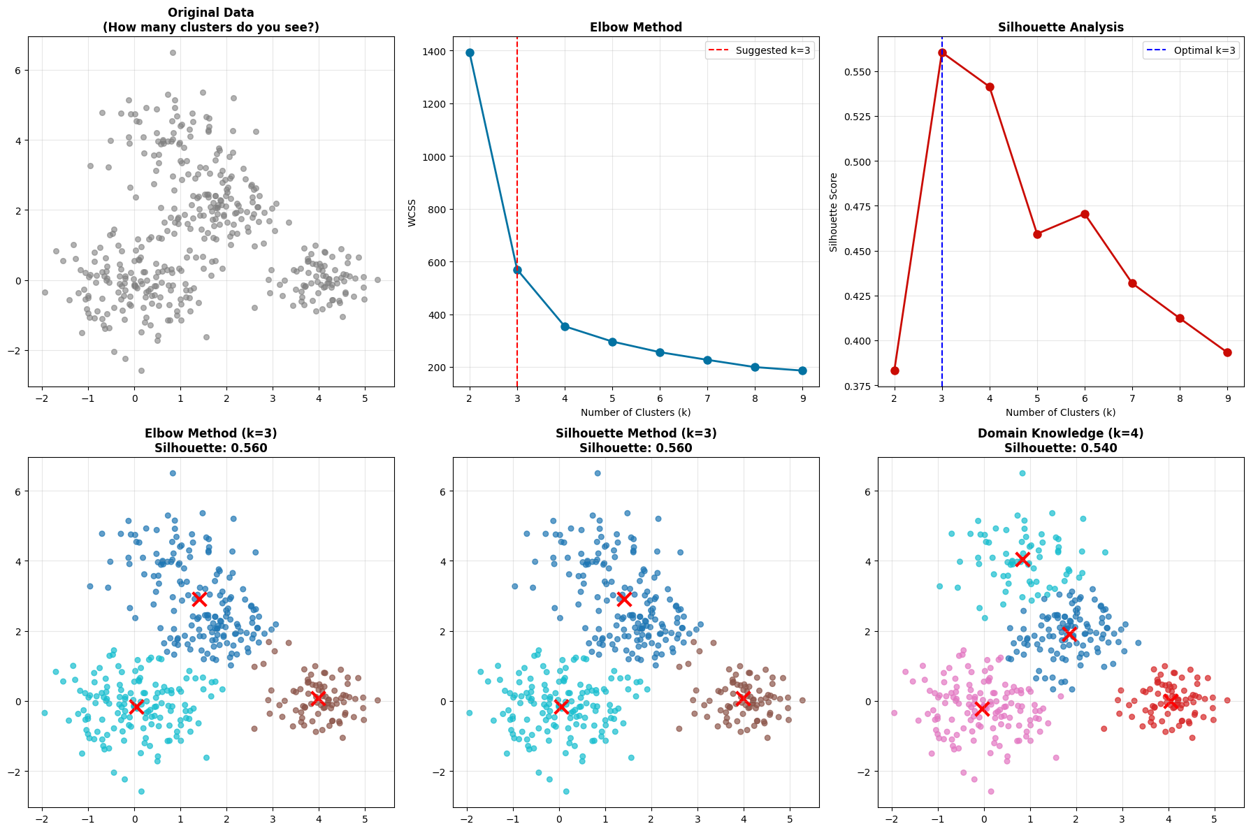
Elbow Method#

Plot WCSS versus K
Look for the “elbow” where improvement diminishes

It’s called the elbow method because the curve looks like an arm, and you’re looking for the elbow joint

Silhouette Analysis#

Measures how similar a point is to its own cluster compared to other clusters
Range from -1 to 1, higher is better
Gives you a quality score for each K value

The Silhouette Coefficient is given by the equation

\(s(i) = \frac{b(i) - a(i)}{\max(a(i), b(i))}\)

Where:

\(a(i)\) = average intra-cluster distance for point \(i\)
\(b(i)\) = average distance to nearest cluster for point \(i\)
Range: \([-1, 1]\) (higher is better)

Look at the output from the code below:

Show code cell source

Hide code cell source

def comprehensive_cluster_analysis(X, max_k=10):
    """Perform both elbow method and silhouette analysis"""

    k_range = range(2, max_k + 1)
    wcss_values = []
    silhouette_scores = []

    print("**Analyzing optimal number of clusters...**")

    # Calculate metrics for each k
    for k in k_range:
        kmeans = KMeans(n_clusters=k, random_state=42, n_init=10)
        labels = kmeans.fit_predict(X)

        wcss_values.append(kmeans.inertia_)
        silhouette_scores.append(silhouette_score(X, labels))

    # Create comprehensive visualization
    fig, axes = plt.subplots(2, 2, figsize=(15, 10))

    # Elbow plot
    axes[0, 0].plot(k_range, wcss_values, 'bo-', linewidth=2, markersize=8)
    axes[0, 0].set_xlabel('Number of Clusters (k)')
    axes[0, 0].set_ylabel('Within-Cluster Sum of Squares (WCSS)')
    axes[0, 0].set_title('Elbow Method', fontweight='bold')
    axes[0, 0].grid(True, alpha=0.3)

    # Silhouette plot
    axes[0, 1].plot(k_range, silhouette_scores, 'ro-', linewidth=2, markersize=8)
    axes[0, 1].set_xlabel('Number of Clusters (k)')
    axes[0, 1].set_ylabel('Silhouette Score')
    axes[0, 1].set_title('Silhouette Analysis', fontweight='bold')
    axes[0, 1].grid(True, alpha=0.3)

    # Mark optimal points
    optimal_silhouette_k = k_range[np.argmax(silhouette_scores)]
    axes[0, 1].axvline(x=optimal_silhouette_k, color='red', linestyle='--',
                      label=f'Optimal k={optimal_silhouette_k}')
    axes[0, 1].legend()

    # Show results with different k values
    test_k_values = [3, 5, 7]
    for idx, k in enumerate(test_k_values[:2]):
        ax = axes[1, idx]
        kmeans = KMeans(n_clusters=k, random_state=42)
        labels = kmeans.fit_predict(X)

        scatter = ax.scatter(X[:, 0], X[:, 1], c=labels, cmap='tab10', alpha=0.7, s=30)
        ax.scatter(kmeans.cluster_centers_[:, 0], kmeans.cluster_centers_[:, 1],
                  c='red', marker='x', s=200, linewidths=3, label='Centroids')

        sil_score = silhouette_score(X, labels)
        ax.set_title(f'k={k}, Silhouette={sil_score:.3f}', fontweight='bold')
        ax.legend()
        ax.grid(True, alpha=0.3)

    plt.tight_layout()
    plt.show()

    return optimal_silhouette_k, max(silhouette_scores)

# Apply to our cybersecurity data
optimal_k, best_silhouette = comprehensive_cluster_analysis(X_cyber)

print(f"\n**Analysis Results:**")
print(f"Optimal k (silhouette): {optimal_k}")
print(f"Best silhouette score: {best_silhouette:.3f}")
print(f"True number of groups: 5 (3 normal + 2 attacks)")

**Analyzing optimal number of clusters...**

../../_images/7e74a6c9f94f30dc0f45659998b5829c7eeedfb947d968bad42d92f636f4547f.png

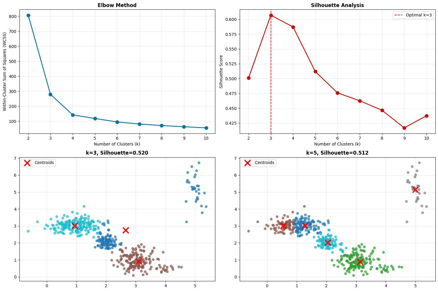
**Analysis Results:**
Optimal k (silhouette): 3
Best silhouette score: 0.607
True number of groups: 5 (3 normal + 2 attacks)

What do you notice? Sometimes the elbow method and silhouette analysis don’t agree! The elbow might suggest K=5, but silhouette peaks at K=3.

This is completely normal and actually an important lesson - clustering is often subjective. There isn’t always a “right” answer. You need to:

Consider your domain knowledge (the cybersecurity context)
Try multiple values and validate results
Use ensemble methods or different algorithms

Accept that there might not be a perfect answer!

When K-means Fails#

K-means makes some strong assumptions:

K-means Assumptions:

Clusters are spherical (circular/elliptical)
Clusters have similar sizes
Clusters have similar densities
All features are equally important

Note

Assumptions Real-world cybersecurity data violates these assumptions all the time!

Look at these three scenarios:#

Non-spherical clusters - Attack campaigns might form crescent or curved patterns. K-means tries to fit spherical clusters and fails.
Different densities - Normal traffic might be very dense (lots of similar flows), while attack traffic is sparse. K-means struggles because it assumes similar densities.
Different sizes - You might have major attack types (many instances) and minor attack types (few instances). K-means tends to split large clusters and merge small ones.

Show code cell source

Hide code cell source

def create_challenging_datasets():
    """Create datasets where K-means struggles"""

    np.random.seed(42)

    # Dataset 1: Non-spherical clusters (attack campaigns)
    t = np.linspace(0, 2*np.pi, 100)
    cluster1 = np.column_stack([3*np.cos(t), np.sin(t)]) + np.random.normal(0, 0.1, (100, 2))
    cluster2 = np.column_stack([np.cos(t), 3*np.sin(t)]) + [4, 4] + np.random.normal(0, 0.1, (100, 2))
    cluster3 = np.random.normal([0, 0], 0.3, (50, 2))
    X_nonspherical = np.vstack([cluster1, cluster2, cluster3])

    # Dataset 2: Different densities (normal vs attack traffic)
    dense_cluster = np.random.normal([2, 2], 0.2, (200, 2))  # Dense normal traffic
    sparse_cluster = np.random.normal([5, 5], 1.0, (50, 2))   # Sparse attack traffic
    X_diff_density = np.vstack([dense_cluster, sparse_cluster])

    # Dataset 3: Different sizes (major vs minor attack types)
    large_cluster = np.random.normal([1, 1], 0.5, (300, 2))
    small_cluster = np.random.normal([4, 4], 0.3, (30, 2))
    X_diff_sizes = np.vstack([large_cluster, small_cluster])

    return X_nonspherical, X_diff_density, X_diff_sizes

def compare_kmeans_performance(datasets, titles, true_k_values):
    """Compare K-means performance on challenging datasets"""

    fig, axes = plt.subplots(2, 3, figsize=(18, 12))

    for idx, (X, title, k) in enumerate(zip(datasets, titles, true_k_values)):
        # Original data
        axes[0, idx].scatter(X[:, 0], X[:, 1], c='gray', alpha=0.6, s=30)
        axes[0, idx].set_title(f'Original: {title}', fontweight='bold')
        axes[0, idx].grid(True, alpha=0.3)

        # K-means results
        kmeans = KMeans(n_clusters=k, random_state=42)
        labels = kmeans.fit_predict(X)

        scatter = axes[1, idx].scatter(X[:, 0], X[:, 1], c=labels, cmap='tab10', alpha=0.7, s=30)
        axes[1, idx].scatter(kmeans.cluster_centers_[:, 0], kmeans.cluster_centers_[:, 1],
                           c='red', marker='x', s=200, linewidths=3)

        sil_score = silhouette_score(X, labels)
        axes[1, idx].set_title(f'K-means (k={k})\nSilhouette: {sil_score:.3f}', fontweight='bold')
        axes[1, idx].grid(True, alpha=0.3)

    plt.tight_layout()
    plt.show()

# Create and analyze challenging datasets
print("**When K-means Struggles: Cybersecurity Scenarios**")

X_nonspherical, X_diff_density, X_diff_sizes = create_challenging_datasets()

datasets = [X_nonspherical, X_diff_density, X_diff_sizes]
titles = ['Attack Campaigns (Non-spherical)', 'Traffic Densities (Variable)', 'Attack Types (Different sizes)']
k_values = [3, 2, 2]

compare_kmeans_performance(datasets, titles, k_values)

print("\n**Key Insight**: K-means assumes spherical, similar-sized clusters")
print("**Cybersecurity Reality**: Attack patterns are often irregular and varied")

**When K-means Struggles: Cybersecurity Scenarios**

../../_images/de3109c4ef7611200376347fc6751aa128ae63465f4a5bf692d3b65841ade2c8.png

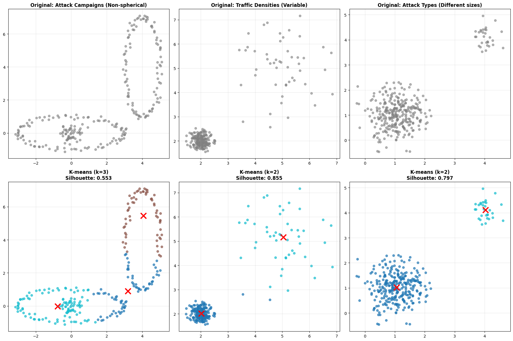
**Key Insight**: K-means assumes spherical, similar-sized clusters
**Cybersecurity Reality**: Attack patterns are often irregular and varied

Note

Key Insight K-means assumes spherical, similar-sized clusters. In reality attack patterns are often irregular and varied.

This is why we need more sophisticated methods.

Gaussian Mixture Models - Adding Flexibility#

GMM takes a probabilistic approach. Instead of saying “this point belongs to cluster A,” it says “this point has a 70% probability of belonging to cluster A and 30% probability of belonging to cluster B.”

Mathematical Foundation#

Note

The Assumption GMM assumes your data comes from a mixture of Gaussian (normal) distributions.

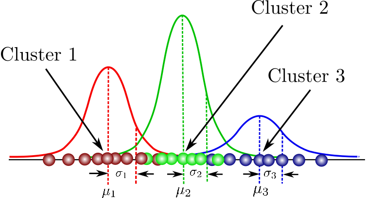
In a GMM each cluster is defined by:

A mean (\(\mu\)) - the center
A covariance matrix (\(\sigma\)) - the shape and orientation
A mixing coefficient (\(\pi\)) - how prevalent this cluster is

This flexibility allows GMM to model elliptical clusters with different shapes and orientations. One of the key advantages of a GMM is that it defines a probaility density function given by:

\[p(x) = \sum_{k=1}^{K} \pi_k \mathcal{N}(x | \mu_k, \sigma_k)\]

Where:

\(\pi_k\) = mixing coefficient (weight) for component \(k\)
\(\mathcal{N}(x | \mu_k, \sigma_k)\) = multivariate Gaussian with mean \(\mu_k\) and covariance \(\sigma_k\)
\(\sum_{k=1}^{K} \pi_k = 1\)

This enables you to set a liklihood threshold instead of a distance threshold when identifying if a certain event should be considered normal or abnormal.

THe Key Advantages over K-means#

Soft clustering: Points can belong to multiple clusters with probabilities
Flexible shapes: Elliptical clusters (not just circular)
Variable sizes: Different cluster covariances mean clusters can be different sizes and shapes. Look back at the previous embeddings of CICIIDS dataset to see that clusters have a high degree of variance
Uncertainty quantification: Probability of cluster membership. This tells you when the model is uncertain, which is valuable information.

GMM vs K-means Comparison#

Show code cell source

Hide code cell source

def demonstrate_gmm_vs_kmeans(X):
    """Compare GMM and K-means on the same data"""

    # Apply both methods
    k = 3

    # K-means
    kmeans = KMeans(n_clusters=k, random_state=42)
    kmeans_labels = kmeans.fit_predict(X)

    # GMM
    gmm = GaussianMixture(n_components=k, random_state=42)
    gmm.fit(X)
    gmm_labels = gmm.predict(X)
    gmm_probs = gmm.predict_proba(X)

    # Visualization
    fig, axes = plt.subplots(2, 2, figsize=(15, 12))

    # K-means hard clustering
    scatter = axes[0, 0].scatter(X[:, 0], X[:, 1], c=kmeans_labels, cmap='tab10', alpha=0.7, s=50)
    axes[0, 0].scatter(kmeans.cluster_centers_[:, 0], kmeans.cluster_centers_[:, 1],
                      c='red', marker='x', s=200, linewidths=3, label='Centroids')
    axes[0, 0].set_title('K-means (Hard Clustering)', fontweight='bold')
    axes[0, 0].legend()
    axes[0, 0].grid(True, alpha=0.3)

    # GMM hard clustering
    scatter = axes[0, 1].scatter(X[:, 0], X[:, 1], c=gmm_labels, cmap='tab10', alpha=0.7, s=50)
    axes[0, 1].scatter(gmm.means_[:, 0], gmm.means_[:, 1],
                      c='red', marker='x', s=200, linewidths=3, label='Means')
    axes[0, 1].set_title('GMM (Hard Clustering)', fontweight='bold')
    axes[0, 1].legend()
    axes[0, 1].grid(True, alpha=0.3)

    # GMM soft clustering - show uncertainty
    # Use maximum probability as color intensity
    max_probs = np.max(gmm_probs, axis=1)
    scatter = axes[1, 0].scatter(X[:, 0], X[:, 1], c=gmm_labels, cmap='tab10',
                               alpha=max_probs, s=50)  # Alpha shows certainty
    axes[1, 0].set_title('GMM (Soft Clustering)\nTransparency = Uncertainty', fontweight='bold')
    axes[1, 0].grid(True, alpha=0.3)

    # Show probability distributions for each component
    for i in range(k):
        component_probs = gmm_probs[:, i]
        scatter = axes[1, 1].scatter(X[:, 0], X[:, 1], c=component_probs,
                                   cmap='viridis', alpha=0.7, s=50)
        if i == 0:  # Only show colorbar for first component
            plt.colorbar(scatter, ax=axes[1, 1], label='Probability')
    axes[1, 1].set_title(f'GMM Component Probabilities\n(Color = P(Component 1))', fontweight='bold')
    axes[1, 1].grid(True, alpha=0.3)

    plt.tight_layout()
    plt.show()

    # Compare performance
    kmeans_sil = silhouette_score(X, kmeans_labels)
    gmm_sil = silhouette_score(X, gmm_labels)

    print(f"\n**Performance Comparison:**")
    print(f"K-means Silhouette: {kmeans_sil:.3f}")
    print(f"GMM Silhouette: {gmm_sil:.3f}")
    print(f"\n**GMM Advantages:**")
    print(f"- Provides uncertainty measures")
    print(f"- Handles elliptical clusters")
    print(f"- Soft cluster assignments")

    return gmm_labels, gmm_probs

# Demonstrate on non-spherical data
print("**GMM vs K-means: Handling Complex Cluster Shapes**")
gmm_labels, gmm_probs = demonstrate_gmm_vs_kmeans(X_nonspherical)

# Show mathematical insight
print(f"\n**Mathematical Insight:**")
print(f"K-means minimizes: Σ||x - μ||²")
print(f"GMM maximizes: Σ log[Σπₖ N(x|μₖ,Σₖ)]")
print(f"Result: GMM can model elliptical clusters with different orientations")

**GMM vs K-means: Handling Complex Cluster Shapes**

../../_images/1760688fa7b312465f984ad7d9e51aa2504e9b8348282ff5b4f5cf3af6e637f8.png

**Performance Comparison:**
K-means Silhouette: 0.553
GMM Silhouette: 0.482

**GMM Advantages:**
- Provides uncertainty measures
- Handles elliptical clusters
- Soft cluster assignments

**Mathematical Insight:**
K-means minimizes: Σ||x - μ||²
GMM maximizes: Σ log[Σπₖ N(x|μₖ,Σₖ)]
Result: GMM can model elliptical clusters with different orientations

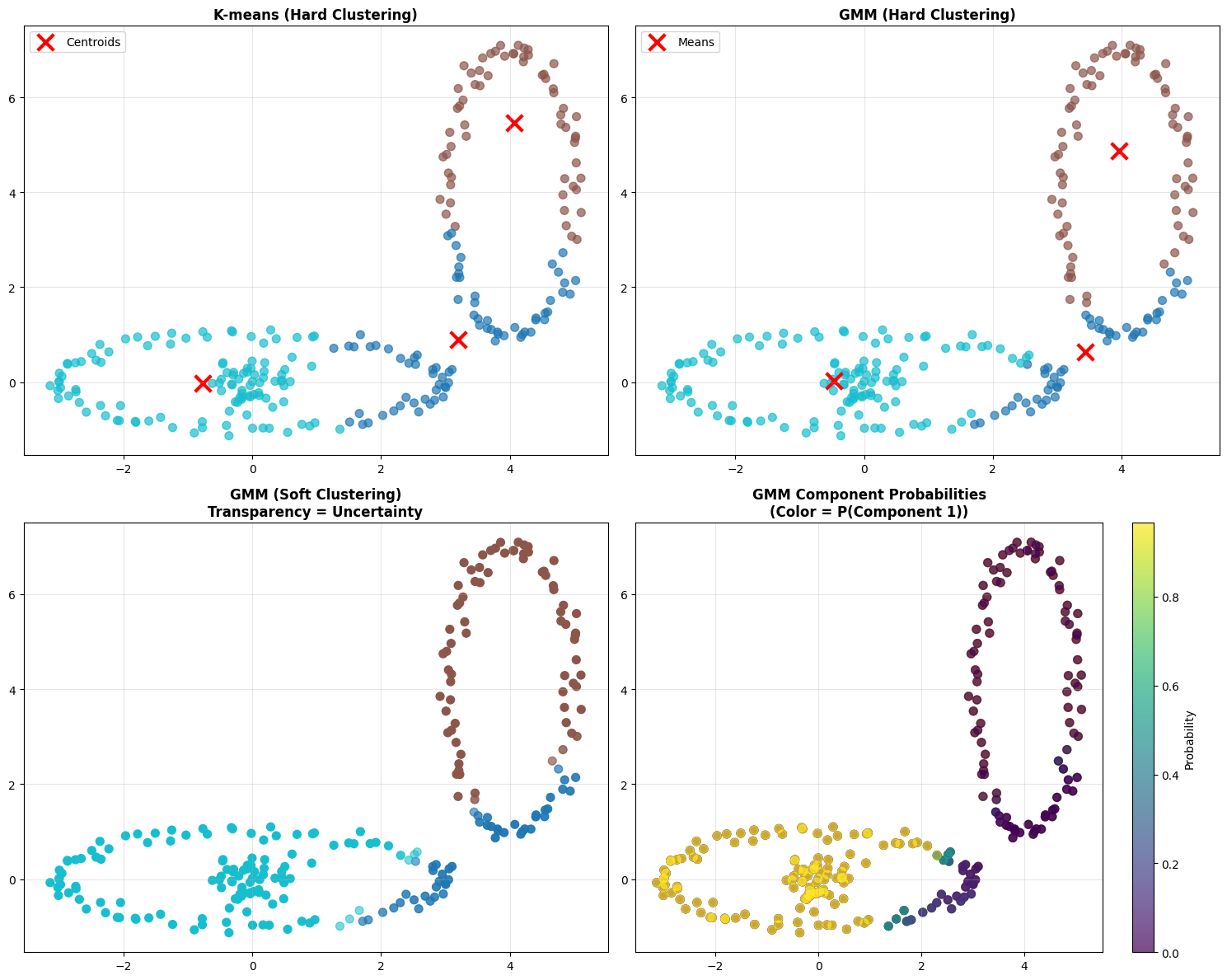
Look at the four plots:

Top left - K-means hard clustering. Each point is definitively assigned to one cluster.
Top right - GMM hard clustering. Using the maximum probability, each point gets a single assignment. Might look similar to K-means at first glance.
Bottom left - GMM soft clustering. The transparency shows certainty. Transparent points are uncertain - they could belong to multiple clusters. Opaque points are definitely in their assigned cluster.
Bottom right - GMM component probabilities. This shows the probability surface for one component. You can see how probability gradually decreases as you move away from the cluster center.

Note

The mathematical insight:

K-means minimizes: Σ||x - μ||²
GMM maximizes: Σ log[Σπₖ N(x|μₖ,Σₖ)]

Result: GMM can model elliptical clusters with different orientations.

The Parameter Selection Dilemma - Again#

Sometimes methods disagree even more dramatically with GMM. GMM typically relies on K-means (default) to initialize the centers. There are other options. such as random or k-means++ which balance initialization speed with convergence quality

Parameter	Default Value	Description
`n_components`	1	Most critical parameter - Number of mixture components/clusters
`covariance_type`	‘full’	Type of covariance: ‘full’ (most flexible), ‘tied’, ‘diag’, or ‘spherical’
`max_iter`	100	Maximum number of iterations
`n_init`	1	Number of initializations to perform (helps avoid local minima)

The GMM models finds the ideal centers through an initialization phase followed by a Refintement using the Expectation-maximization (EM) algorithm.

THe EM Algorithm is based on Baye’s theorem and goes through an iterative two-step process: *1. E-step (Expectation) where it calculate the probability that each data point belongs to each Gaussian (i.e. cluster assignments) or more often called called the posterior probability. It is essentially using Bayes’ rule to determine how much each component “explains” each data point.

M-step (Maximization) where it updates the parameters (i.e. means (cluster centers), covariances, and mixture weights) to maximize log-likelihood given the posterior probabilities calculated in step 1. i.e. we want the model to provide a higher “confidence” that the point belongs to one of the Gaussian Clusters - and we maximize this across all points.

Part 4: DBSCAN - A Different Approach#

Density-Based Spatial Clustering of Applications with Noise or more commonly referred to as DBSCAN is fundamentally different from K-means and GMM. Instead of asking “how many clusters?” it asks “where are the dense regions?

Mathematical Foundation#

There are several Key Concepts to keep in mind:

Core Point: A core point is one with at least a min_samples neighbors within a distance eps. These are considered in the “heart” of the cluster.
Border Point: A Non-core point within the distance eps of a core point
Noise Point: Neither core nor border (potential anomalies!)

Intuitively this would be like looking at a groups of people at a tailgate. If they are within 5 feet of 4 friends then they are a core point in the group. If they are only within 5 feet of 1 or 2 friends within that core group, then they are still in the group, but on the edge. If they are outside 5 feet, they aren’t in any group.

Mathematical Definitions:

ε-neighborhood: \(N_{\varepsilon}(p) = \{q \in D | dist(p,q) \leq \varepsilon\}\)
Core point: \(|N_{\varepsilon}(p)| \geq MinPts\)
Directly density-reachable: \(q \in N_{\varepsilon}(p)\) and \(p\) is core
Density-reachable: Chain of directly density-reachable points

The Algorithm

Algorithm:

For each unvisited point \(p\):
Find its \(\varepsilon\)-neighborhood (\(N_{\varepsilon}(p)\)) - all points within distance \(\varepsilon\)
If it has at least min_samplesneighbors (\(|N_{\varepsilon}(p)| \geq MinPts\)) then start a new cluster
Add all density-reachable points to cluster
Mark isolated points as noise

Key Advantages:

No need to specify number of clusters
Finds arbitrary cluster shapes, Non-spherical, irregular patterns are fine
Automatically identifies outliers/anomalies
Robust to noise as unlike the other methods it doesn’t try to force every point into a cluster

Key DBSCAN Hyperparameters**#

Parameter	Description	Default	Impact
`eps`	Maximum distance between points	Must specify	Critical: Controls cluster boundaries
`min_samples`	Minimum points in neighborhood	`5`	Major: Determines core/noise classification
`metric`	Distance metric	`'euclidean'`	How distances are calculated
`algorithm`	Neighbor search method	`'auto'`	Performance optimization

The two critical parameters are:

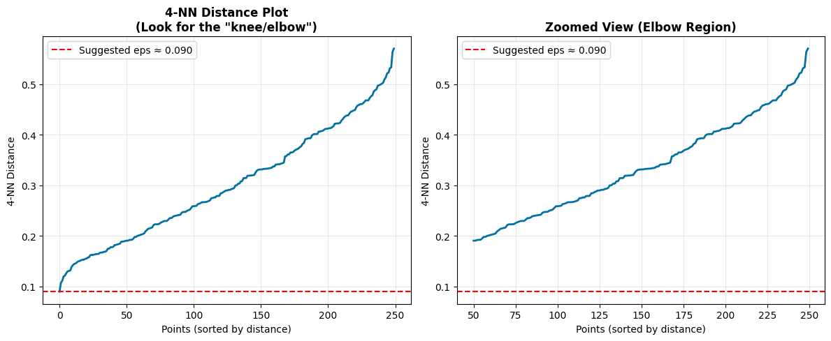
eps - Maximum distance between points in a cluster. Too small, everything is noise. Too large, everything is one cluster.
min_samples - Minimum points to form a dense region. Too small, noise becomes clusters. Too large, real clusters become noise.

Let’s go back to the same dataset we used before and watch what happens when we change eps. With eps=0.3, you might get many small clusters and lots of noise. With eps=1.0, clusters merge together. You’re looking for the sweet spot.

Hint

Hint This is a great place to apply hyperparameter search methods from last class

Show code cell source

Hide code cell source

def demonstrate_dbscan_concepts(X, eps_values=[0.3, 0.6, 1.0], min_samples=5):
    """Visualize DBSCAN concepts and parameter effects"""

    fig, axes = plt.subplots(2, 2, figsize=(15, 12))
    axes = axes.flatten()

    # Original data
    axes[0].scatter(X[:, 0], X[:, 1], c='gray', alpha=0.6, s=50)
    axes[0].set_title('Original Data', fontweight='bold')
    axes[0].grid(True, alpha=0.3)

    # Test different eps values
    for i, eps in enumerate(eps_values):
        if i < 3:  # Only show first 3
            ax = axes[i + 1]

            # Apply DBSCAN
            dbscan = DBSCAN(eps=eps, min_samples=min_samples)
            labels = dbscan.fit_predict(X)

            # Count clusters and noise
            n_clusters = len(set(labels)) - (1 if -1 in labels else 0)
            n_noise = sum(labels == -1)

            # Plot results
            unique_labels = set(labels)
            colors = plt.cm.tab10(np.linspace(0, 1, len(unique_labels)))

            for label, color in zip(unique_labels, colors):
                if label == -1:
                    # Noise points (black x's)
                    mask = labels == label
                    ax.scatter(X[mask, 0], X[mask, 1], c='red', marker='x', s=100,
                              alpha=0.8, label=f'Noise ({n_noise})')
                else:
                    # Cluster points
                    mask = labels == label
                    ax.scatter(X[mask, 0], X[mask, 1], c=[color], s=50, alpha=0.7,
                              label=f'Cluster {label}')

            ax.set_title(f'DBSCAN: eps={eps}, min_samples={min_samples}\n'
                        f'Clusters: {n_clusters}, Noise: {n_noise}', fontweight='bold')
            ax.grid(True, alpha=0.3)
            ax.legend()

    plt.tight_layout()
    plt.show()

    return labels

def find_optimal_eps(X, min_samples=5):
    """Find optimal eps using k-NN distance plot"""

    print(f"\n**Finding Optimal eps Parameter**")
    print(f"Method: k-NN distance plot (k = min_samples - 1 = {min_samples-1})")

    # Calculate k-NN distances
    k = min_samples - 1
    neighbors = NearestNeighbors(n_neighbors=k + 1)  # +1 because point is its own neighbor
    neighbors.fit(X)
    distances, indices = neighbors.kneighbors(X)

    # Get k-th nearest neighbor distances (excluding self)
    k_distances = distances[:, k]
    k_distances = np.sort(k_distances)

    # Plot k-NN distance plot
    plt.figure(figsize=(12, 5))

    plt.subplot(1, 2, 1)
    plt.plot(k_distances, 'b-', linewidth=2)
    plt.xlabel('Points (sorted by distance)')
    plt.ylabel(f'{k}-NN Distance')
    plt.title(f'{k}-NN Distance Plot\n(Look for the "knee/elbow")', fontweight='bold')
    plt.grid(True, alpha=0.3)

    # Suggest eps value (where curve starts to rise steeply)
    # Find point where gradient increases significantly
    gradients = np.gradient(k_distances)
    steep_start = np.where(gradients > np.percentile(gradients, 95))[0]

    if len(steep_start) > 0:
        suggested_eps = k_distances[steep_start[0]]
        plt.axhline(y=suggested_eps, color='red', linestyle='--',
                   label=f'Suggested eps ≈ {suggested_eps:.3f}')
        plt.legend()
    else:
        suggested_eps = np.percentile(k_distances, 95)

    # Show zoomed view
    plt.subplot(1, 2, 2)
    zoom_start = max(0, len(k_distances) - 200)
    plt.plot(range(zoom_start, len(k_distances)), k_distances[zoom_start:], 'b-', linewidth=2)
    plt.axhline(y=suggested_eps, color='red', linestyle='--',
               label=f'Suggested eps ≈ {suggested_eps:.3f}')
    plt.xlabel('Points (sorted by distance)')
    plt.ylabel(f'{k}-NN Distance')
    plt.title('Zoomed View (Elbow Region)', fontweight='bold')
    plt.legend()
    plt.grid(True, alpha=0.3)

    plt.tight_layout()
    plt.show()

    return suggested_eps

# Demonstrate DBSCAN on challenging data
print("**DBSCAN: Handling Complex Cluster Shapes**")
print("Perfect for cybersecurity data with irregular attack patterns!")

# Use non-spherical data to show DBSCAN's strength
dbscan_labels = demonstrate_dbscan_concepts(X_nonspherical)

# Find optimal parameters
optimal_eps = find_optimal_eps(X_nonspherical)

print(f"\n**DBSCAN Key Advantages for Cybersecurity:**")
print(f"✓ No need to specify number of attack types (clusters)")
print(f"✓ Finds irregular attack patterns (non-spherical clusters)")
print(f"✓ Automatically identifies anomalies (noise points)")
print(f"✓ Robust to outliers in normal traffic")

**DBSCAN: Handling Complex Cluster Shapes**
Perfect for cybersecurity data with irregular attack patterns!

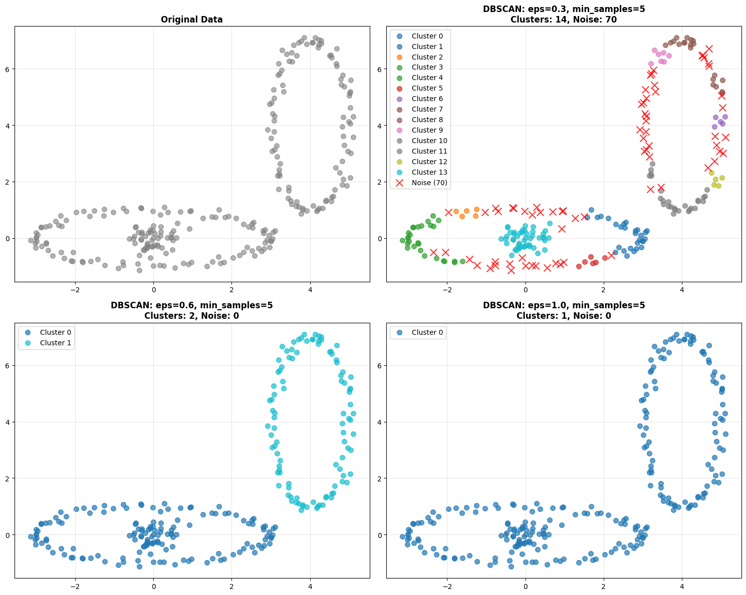
../../_images/24c4841ba883e30f241b23f26b88888af4e3eaf1a9a9ff2befb99b83818e7a69.png

**Finding Optimal eps Parameter**
Method: k-NN distance plot (k = min_samples - 1 = 4)

../../_images/bb04f52ae78ad6847bb11cbbaf0b78ccecaabdad91c41d607802bf770980b796.png

**DBSCAN Key Advantages for Cybersecurity:**
✓ No need to specify number of attack types (clusters)
✓ Finds irregular attack patterns (non-spherical clusters)
✓ Automatically identifies anomalies (noise points)
✓ Robust to outliers in normal traffic

Comprehensive Method Comparison#

Now let’s compare all three methods on the same dataset to understand their strengths and weaknesses.

Hint

Explore how changing the parameters such as k, eps, etc. impacts the output. This dataset is intentionally spherical with some outlier noise.

Show code cell source

Hide code cell source

def comprehensive_method_comparison(X):
    """Compare K-means, GMM, and DBSCAN on the same dataset"""

    print("**Comprehensive Method Comparison**")
    print("Testing all three methods on complex cybersecurity-like data...")

    # Apply all three methods
    k = 4  # Reasonable guess for number of clusters

    # K-means
    kmeans = KMeans(n_clusters=k, random_state=42)
    kmeans_labels = kmeans.fit_predict(X)

    # GMM
    gmm = GaussianMixture(n_components=k, random_state=42)
    gmm_labels = gmm.fit_predict(X)

    # DBSCAN (use optimal eps from previous analysis)
    dbscan = DBSCAN(eps=0.8, min_samples=5)
    dbscan_labels = dbscan.fit_predict(X)

    # Visualization
    fig, axes = plt.subplots(2, 2, figsize=(15, 12))

    # Original data
    axes[0, 0].scatter(X[:, 0], X[:, 1], c='gray', alpha=0.6, s=30)
    axes[0, 0].set_title('Original Data\n(Complex Patterns)', fontweight='bold')
    axes[0, 0].grid(True, alpha=0.3)

    # K-means results
    axes[0, 1].scatter(X[:, 0], X[:, 1], c=kmeans_labels, cmap='tab10', alpha=0.7, s=30)
    axes[0, 1].scatter(kmeans.cluster_centers_[:, 0], kmeans.cluster_centers_[:, 1],
                      c='red', marker='x', s=200, linewidths=3, label='Centroids')
    kmeans_sil = silhouette_score(X, kmeans_labels)
    axes[0, 1].set_title(f'K-means (k={k})\nSilhouette: {kmeans_sil:.3f}', fontweight='bold')
    axes[0, 1].legend()
    axes[0, 1].grid(True, alpha=0.3)

    # GMM results
    axes[1, 0].scatter(X[:, 0], X[:, 1], c=gmm_labels, cmap='tab10', alpha=0.7, s=30)
    axes[1, 0].scatter(gmm.means_[:, 0], gmm.means_[:, 1],
                      c='red', marker='x', s=200, linewidths=3, label='Means')
    gmm_sil = silhouette_score(X, gmm_labels)
    axes[1, 0].set_title(f'GMM (k={k})\nSilhouette: {gmm_sil:.3f}', fontweight='bold')
    axes[1, 0].legend()
    axes[1, 0].grid(True, alpha=0.3)

    # DBSCAN results
    unique_labels = set(dbscan_labels)
    colors = plt.cm.tab10(np.linspace(0, 1, len(unique_labels)))

    for label, color in zip(unique_labels, colors):
        if label == -1:
            # Noise points
            mask = dbscan_labels == label
            axes[1, 1].scatter(X[mask, 0], X[mask, 1], c='red', marker='x', s=100,
                              alpha=0.8, label=f'Noise ({sum(mask)})')
        else:
            # Cluster points
            mask = dbscan_labels == label
            axes[1, 1].scatter(X[mask, 0], X[mask, 1], c=[color], s=30, alpha=0.7)

    n_clusters_db = len(set(dbscan_labels)) - (1 if -1 in dbscan_labels else 0)
    n_noise = sum(dbscan_labels == -1)

    # Calculate silhouette for DBSCAN (excluding noise points)
    if n_clusters_db > 1:
        non_noise_mask = dbscan_labels != -1
        if sum(non_noise_mask) > 0:
            dbscan_sil = silhouette_score(X[non_noise_mask], dbscan_labels[non_noise_mask])
        else:
            dbscan_sil = -1
    else:
        dbscan_sil = -1

    axes[1, 1].set_title(f'DBSCAN\nClusters: {n_clusters_db}, Noise: {n_noise}\nSilhouette: {dbscan_sil:.3f}',
                        fontweight='bold')
    axes[1, 1].legend()
    axes[1, 1].grid(True, alpha=0.3)

    plt.tight_layout()
    plt.show()

    # Performance summary
    print(f"\n**Method Comparison Summary:**")
    print(f"{'Method':<12} {'Clusters':<10} {'Noise':<8} {'Silhouette':<12} {'Key Strength'}")
    print(f"{'='*65}")
    print(f"{'K-means':<12} {k:<10} {'0':<8} {kmeans_sil:<12.3f} Fast, simple")
    print(f"{'GMM':<12} {k:<10} {'0':<8} {gmm_sil:<12.3f} Probabilistic, flexible shapes")
    print(f"{'DBSCAN':<12} {n_clusters_db:<10} {n_noise:<8} {dbscan_sil:<12.3f} Auto-detects anomalies")

    print(f"\n**Key Insights for Cybersecurity:**")
    print(f"• K-means: Good baseline, assumes spherical attack patterns")
    print(f"• GMM: Better for overlapping/uncertain classifications")
    print(f"• DBSCAN: Ideal when attack patterns are irregular & you need anomaly detection")

    return {
        'kmeans': (kmeans_labels, kmeans_sil),
        'gmm': (gmm_labels, gmm_sil),
        'dbscan': (dbscan_labels, dbscan_sil)
    }

# Run comprehensive comparison
comparison_results = comprehensive_method_comparison(X_cyber)

print(f"\n**Decision Framework for Cybersecurity Applications:**")
print(f"\n**Choose K-means when:**")
print(f"• You have a rough idea of number of attack types")
print(f"• You need fast, interpretable results")
print(f"• Attack patterns are roughly circular/spherical")

print(f"\n**Choose GMM when:**")
print(f"• You need uncertainty quantification")
print(f"• Attack patterns have different shapes/orientations")
print(f"• You want soft cluster assignments")

print(f"\n**Choose DBSCAN when:**")
print(f"• Unknown number of attack types")
print(f"• Irregular attack patterns expected")
print(f"• Automatic anomaly detection is priority")
print(f"• Robust outlier handling needed")

**Comprehensive Method Comparison**
Testing all three methods on complex cybersecurity-like data...

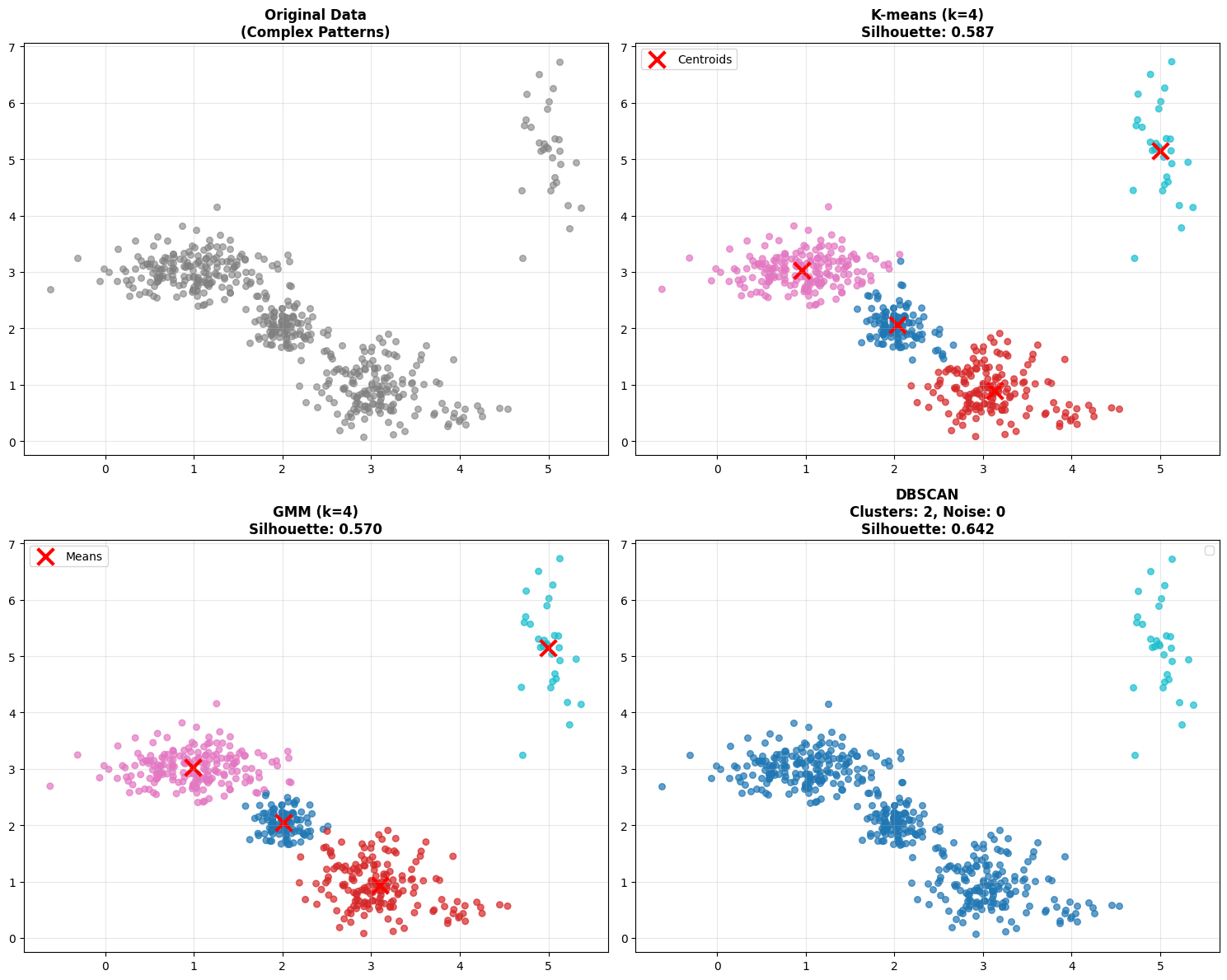
../../_images/edc549cd662abbd4f193fc45abe21245b7ea3c840e71658b9c388a991e3320a7.png

**Method Comparison Summary:**
Method       Clusters   Noise    Silhouette   Key Strength
=================================================================
K-means      4          0        0.587        Fast, simple
GMM          4          0        0.570        Probabilistic, flexible shapes
DBSCAN       2          0        0.642        Auto-detects anomalies

**Key Insights for Cybersecurity:**
• K-means: Good baseline, assumes spherical attack patterns
• GMM: Better for overlapping/uncertain classifications
• DBSCAN: Ideal when attack patterns are irregular & you need anomaly detection

**Decision Framework for Cybersecurity Applications:**

**Choose K-means when:**
• You have a rough idea of number of attack types
• You need fast, interpretable results
• Attack patterns are roughly circular/spherical

**Choose GMM when:**
• You need uncertainty quantification
• Attack patterns have different shapes/orientations
• You want soft cluster assignments

**Choose DBSCAN when:**
• Unknown number of attack types
• Irregular attack patterns expected
• Automatic anomaly detection is priority
• Robust outlier handling needed

Check out the table that’s printed. You’ll see silhouette scores for each method. But don’t just look at the numbers - look at the actual clustering results. Sometimes a lower silhouette score is acceptable if the method is finding more meaningful clusters for your application. or in this case if your data is noisy.

Next Steps and Advanced Methods#

The Clustering Algorithm Landscape#

Today we covered three fundamental approaches but the clustering landscape is much larger:

Centroid-based: K-means, K-medoids, k-modes
Distribution-based: Gaussian Mixture Models (GMM)
Density-based: DBSCAN, OPTICS, HDBSCAN
Hierarchical: Agglomerative, Divisive
Graph-based: Spectral clustering
And many more…

Each has its place in the toolkit. Often times finding the right one is more art than science. EDA and exploration (i.e. trial and error) are your friend.

When Traditional Clustering Isn’t Enough#

The “Normal Behavior” Problem in Cybersecurity:

Network behavior changes constantly
Seasonal patterns (business hours, weekends)
Evolution of legitimate applications
New types of normal behavior emerge

Traditional clustering limitations:

Static models don’t adapt
High-dimensional feature spaces
Temporal dependencies ignored
Complex behavioral patterns

Look at this time-series visualization below. The color represents time. Notice how the “normal” behavior drifts over time? The static K-means model, trained on early data, becomes outdated. It may start flagging new normal behavior as anomalies because the model hasn’t adapted.

This is the motivation for next week’s topic: Deep Learning.

Show code cell source

Hide code cell source

# Demonstrate the "normal behavior" challenge
def demonstrate_evolving_behavior():
    """Show how normal behavior can evolve over time"""

    print("**The Challenge: Evolving Normal Behavior**")

    # Simulate network behavior over time
    np.random.seed(42)
    time_points = np.linspace(0, 4*np.pi, 300)

    # Base normal behavior that shifts over time
    normal_x = 2 + 0.5 * np.sin(time_points) + np.random.normal(0, 0.2, 300)
    normal_y = 2 + 0.3 * np.cos(time_points) + np.random.normal(0, 0.2, 300)

    # Add some attacks (fixed pattern)
    attack_x = np.array([4, 4.1, 3.9, 4.2] * 10)[:40]
    attack_y = np.array([4, 4.2, 3.8, 4.1] * 10)[:40]
    attack_times = np.random.choice(range(300), 40, replace=False)

    # Combine data
    X_evolving = np.column_stack([normal_x, normal_y])
    X_evolving[attack_times] = np.column_stack([attack_x, attack_y])

    # Show how static clustering fails
    fig, axes = plt.subplots(1, 3, figsize=(18, 6))

    # Time-colored plot
    scatter = axes[0].scatter(X_evolving[:, 0], X_evolving[:, 1],
                             c=time_points, cmap='viridis', alpha=0.7, s=30)
    axes[0].scatter(X_evolving[attack_times, 0], X_evolving[attack_times, 1],
                   c='red', marker='x', s=100, alpha=0.8, label='Attacks')
    plt.colorbar(scatter, ax=axes[0], label='Time')
    axes[0].set_title('Evolving Normal Behavior\n(Color = Time)', fontweight='bold')
    axes[0].legend()
    axes[0].grid(True, alpha=0.3)

    # Static K-means (trained on early data)
    early_data = X_evolving[:100]  # Train on first 100 points
    kmeans_static = KMeans(n_clusters=2, random_state=42)
    early_labels = kmeans_static.fit_predict(early_data)

    # Apply to all data
    all_labels_static = kmeans_static.predict(X_evolving)

    axes[1].scatter(X_evolving[:, 0], X_evolving[:, 1],
                   c=all_labels_static, cmap='tab10', alpha=0.7, s=30)
    axes[1].scatter(kmeans_static.cluster_centers_[:, 0], kmeans_static.cluster_centers_[:, 1],
                   c='red', marker='x', s=200, linewidths=3, label='Static Centroids')
    axes[1].scatter(X_evolving[attack_times, 0], X_evolving[attack_times, 1],
                   c='black', marker='s', s=50, alpha=0.8, label='True Attacks')
    axes[1].set_title('Static K-means\n(Trained on Early Data)', fontweight='bold')
    axes[1].legend()
    axes[1].grid(True, alpha=0.3)

    # Show the problem
    axes[2].text(0.1, 0.7, 'Problems with Static Models:', fontsize=14, fontweight='bold',
                transform=axes[2].transAxes)
    axes[2].text(0.1, 0.6, '• Normal behavior drifts over time', fontsize=12,
                transform=axes[2].transAxes)
    axes[2].text(0.1, 0.5, '• Static centroids become outdated', fontsize=12,
                transform=axes[2].transAxes)
    axes[2].text(0.1, 0.4, '• False positives increase', fontsize=12,
                transform=axes[2].transAxes)
    axes[2].text(0.1, 0.3, '• New normal patterns seen as attacks', fontsize=12,
                transform=axes[2].transAxes)

    axes[2].text(0.1, 0.15, 'Solutions:', fontsize=14, fontweight='bold', color='blue',
                transform=axes[2].transAxes)
    axes[2].text(0.1, 0.05, '• Deep Learning (Autoencoders, VAEs)', fontsize=12, color='blue',
                transform=axes[2].transAxes)
    axes[2].set_xlim(0, 1)
    axes[2].set_ylim(0, 1)
    axes[2].axis('off')

    plt.tight_layout()
    plt.show()

    print("\n**The Evolution Challenge:**")
    print("• Normal behavior patterns change over time")
    print("• Static clustering models become outdated")
    print("• Need adaptive, continuous learning approaches")
    print("• Traditional methods struggle with high-dimensional, temporal data")

demonstrate_evolving_behavior()

print("\n\n" + "="*60)
print("**PREVIEW: NEXT WEEK - DEEP LEARNING APPROACHES**")
print("="*60)

print("\n**Why Deep Learning for Cybersecurity?**")
print("• Handle high-dimensional feature spaces automatically")
print("• Learn complex, non-linear patterns in data")
print("• Adapt to evolving normal behavior")
print("• Model temporal dependencies and sequences")

print("\n**Methods we'll explore:**")
print("• **Autoencoders**: Learn compressed representations of normal behavior")
print("• **Variational Autoencoders (VAEs)**: Probabilistic generative models")
print("• **Recurrent Neural Networks**: For temporal/sequential patterns")
print("• **Graph Neural Networks**: For network topology analysis")

print("\n**Real-world applications:**")
print("• Advanced Persistent Threat (APT) detection")
print("• Zero-day malware identification")
print("• Insider threat detection")
print("• Network intrusion detection systems")

print(f"\n**Today's Foundation + Next Week's Power = Advanced Cybersecurity AI**")

**The Challenge: Evolving Normal Behavior**

../../_images/91ddf2b757754b25feb102ac2f42ab7dab77aa8ebeb75dcc3d91f00e13a60a9c.png

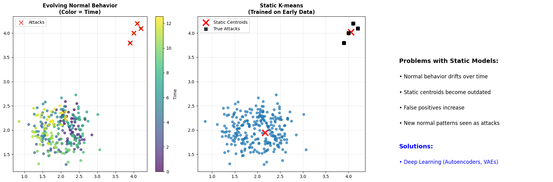
**The Evolution Challenge:**
• Normal behavior patterns change over time
• Static clustering models become outdated
• Need adaptive, continuous learning approaches
• Traditional methods struggle with high-dimensional, temporal data


============================================================
**PREVIEW: NEXT WEEK - DEEP LEARNING APPROACHES**
============================================================

**Why Deep Learning for Cybersecurity?**
• Handle high-dimensional feature spaces automatically
• Learn complex, non-linear patterns in data
• Adapt to evolving normal behavior
• Model temporal dependencies and sequences

**Methods we'll explore:**
• **Autoencoders**: Learn compressed representations of normal behavior
• **Variational Autoencoders (VAEs)**: Probabilistic generative models
• **Recurrent Neural Networks**: For temporal/sequential patterns
• **Graph Neural Networks**: For network topology analysis

**Real-world applications:**
• Advanced Persistent Threat (APT) detection
• Zero-day malware identification
• Insider threat detection
• Network intrusion detection systems

**Today's Foundation + Next Week's Power = Advanced Cybersecurity AI**

Summary: Key Takeaways#

Mathematical Progression#

K-means: \(\min \sum_{i=1}^{k} \sum_{x \in C_i} ||x - \mu_i||^2\) (Euclidean distance)
GMM: \(\max \sum_{i=1}^{n} \log \sum_{k=1}^{K} \pi_k \mathcal{N}(x_i | \mu_k, \sigma_k)\) (Probabilistic)
DBSCAN: Density-based, no global optimization function

Method Selection Framework#

Scenario	Method	Reason
Known attack types, regular patterns	K-means	Fast, interpretable
Uncertain classifications, overlapping	GMM	Probabilistic assignments
Unknown threats, irregular patterns	DBSCAN	Auto-detects anomalies
Evolving behavior, high-dimensional	Deep Learning	Adaptive, complex patterns

Cybersecurity Insights#

No perfect clustering method - context and domain knowledge matter
Parameter selection is critical - elbow/silhouette methods provide guidance
Traditional clustering has limits - evolving threats need adaptive approaches
Next frontier: Deep learning for complex, temporal cybersecurity patterns

Next Session: Deep Learning approaches for advanced cybersecurity threat detection

Activity: Hands-on comparison of all three methods on real cybersecurity datasets (See Canvas)

Class 3: Clustering Algorithms for Cybersecurity

Contents

Class 3: Clustering Algorithms for Cybersecurity#

Learning Objectives#

Overview#

The Reality of Real-World Data#

The “Unknown Unknowns” Framework#

Why Traditional Detection is Failing#

Real-World Impact#

NotPetya (2017)#

SolarWinds (2020)#

Volt Typhoon (2023)#

Enter Unsupervised Learning#

Clustering Approach#

Clustering Philosophies#

Centroid-Based: K-means#

Distribution-Based: Gaussian Mixture Models (GMM)#

Density-Based: DBSCAN#

Setup and Imports#

Visualizing the Problem#

K-means Clustering#

The Mathematical Foundation#

Key K-Means Hyperparameters#

The Parameter Selection Challenge#

Elbow Method#

Silhouette Analysis#

When K-means Fails#

Look at these three scenarios:#

Gaussian Mixture Models - Adding Flexibility#

Mathematical Foundation#

THe Key Advantages over K-means#

GMM vs K-means Comparison#

The Parameter Selection Dilemma - Again#

Part 4: DBSCAN - A Different Approach#

Mathematical Foundation#

Key DBSCAN Hyperparameters**#

Comprehensive Method Comparison#

Next Steps and Advanced Methods#

The Clustering Algorithm Landscape#

When Traditional Clustering Isn’t Enough#

Summary: Key Takeaways#

Mathematical Progression#

Method Selection Framework#

Cybersecurity Insights#